Python – XGBoostで回帰分析(Scikit-learn)
今回は業務にて非常に使用する機会の多い、Python – XGBoostで回帰分析(Scikit-learn)について記載していこうと思います。最近では、Causal Inferenceのmodelでもかなり頻繁に使用する機会が多いのではないでしょうか。そこで、今回は回帰/Regressionについて記載していきます。
1. データ準備
データ準備として、今回はsklearn.datasetsのcalifornia_housingを使用していきます。このデータは回帰用のSampleデータとして使用できますので、必要に応じて使用してみてください。また、pandas.dataframeを使用するので、pandasもimportし、sklearn.datasetsのcalifornia_housingのデータをpandas.dataframeに格納します。
In [1]: import pandas as pd
   ...: import numpy as np
   ...: import matplotlib.pyplot as plt
   ...: from sklearn.datasets import fetch_california_housing

In [2]: california_housing = fetch_california_housing()
   ...: df = pd.DataFrame(california_housing.data, columns=california_housing.feature_names)
   ...: df.head()

Out[2]:
   MedInc  HouseAge  AveRooms  AveBedrms  Population  AveOccup  Latitude  Longitude
0  8.3252      41.0  6.984127   1.023810       322.0  2.555556     37.88    -122.23
1  8.3014      21.0  6.238137   0.971880      2401.0  2.109842     37.86    -122.22
2  7.2574      52.0  8.288136   1.073446       496.0  2.802260     37.85    -122.24
3  5.6431      52.0  5.817352   1.073059       558.0  2.547945     37.85    -122.25
4  3.8462      52.0  6.281853   1.081081       565.0  2.181467     37.85    -122.25
california_housingのtargetデータ「MudHouseVal」をpandas.dataframeに追加してデータ準備完了です。
In [3]: df['MedHouseVal'] = pd.Series(california_housing.target)
   ...: df.head()

Out[3]:
   MedInc  HouseAge  AveRooms  AveBedrms  Population  AveOccup  Latitude  Longitude  MedHouseVal
0  8.3252      41.0  6.984127   1.023810       322.0  2.555556     37.88    -122.23        4.526
1  8.3014      21.0  6.238137   0.971880      2401.0  2.109842     37.86    -122.22        3.585
2  7.2574      52.0  8.288136   1.073446       496.0  2.802260     37.85    -122.24        3.521
3  5.6431      52.0  5.817352   1.073059       558.0  2.547945     37.85    -122.25        3.413
4  3.8462      52.0  6.281853   1.081081       565.0  2.181467     37.85    -122.25        3.422
以上でデータ準備は完了です。
2. Training / Validationデータ作成
では、TrainingデータとValidationデータを作成して、modelingの準備をしていこうと思います。
念の為、TargetデータにNaNが存在するかを確認してみます。
In [4]: df['MedHouseVal'].isnull().sum()

Out[4]:
0
特に前処理の必要はなさそうなので、そのまま変数yに代入していきます。
In [5]: y = df['MedHouseVal']次に、Feature setを変数Xに格納し、各カラムの要約統計量を確認してみます。
In [6]: X = df.drop('MedHouseVal', axis=1)
   ...: X.describe()

Out[6]:
             MedInc      HouseAge      AveRooms     AveBedrms    Population      AveOccup      Latitude     Longitude
count  20640.000000  20640.000000  20640.000000  20640.000000  20640.000000  20640.000000  20640.000000  20640.000000
mean       3.870671     28.639486      5.429000      1.096675   1425.476744      3.070655     35.631861   -119.569704
std        1.899822     12.585558      2.474173      0.473911   1132.462122     10.386050      2.135952      2.003532
min        0.499900      1.000000      0.846154      0.333333      3.000000      0.692308     32.540000   -124.350000
25%        2.563400     18.000000      4.440716      1.006079    787.000000      2.429741     33.930000   -121.800000
50%        3.534800     29.000000      5.229129      1.048780   1166.000000      2.818116     34.260000   -118.490000
75%        4.743250     37.000000      6.052381      1.099526   1725.000000      3.282261     37.710000   -118.010000
max       15.000100     52.000000    141.909091     34.066667  35682.000000   1243.333333     41.950000   -114.310000
また、Nullチェックも行います。
In [7]: X.isnull().sum()
Out[7]:
MedInc        0
HouseAge      0
AveRooms      0
AveBedrms     0
Population    0
AveOccup      0
Latitude      0
Longitude     0
dtype: int64
Nullもなさそうなので、Training / Validationデータを作成していきます。
In [8]: from sklearn.model_selection import train_test_split
   ...:
   ...: X_train, X_test, y_train, y_test = train_test_split(X, y, test_size=0.3, random_state=0)
今回は、7:3で作成していますが、業務に合わせて適宜変更することが必要だと思います。
3. XGBoostで回帰分析(Scikit-learn)
それでは、本題の回帰分析を行なっていこうと思います。今回はscikit-learnのxgboostで回帰分析を行なってみます。XGBoost APIでの回帰分析は以下をご参照ください。
3-1. Training
では、XGBoost (scikit-learn API)をimportしてから、trainingを行なっていきます。scikit-learnのXGBoostではDMatrixへの変換が不要なのでXGBRegressor()をインスタンス化し、fit()を行なっていきます。
https://xgboost.readthedocs.io/en/stable/python/python_api.html#xgboost.XGBRegressor
In [9]: from xgboost import XGBRegressor

In [10]: xgb_model1 = XGBRegressor()
    ...: xgb_model1.fit(X_train, y_train, verbose=False)

Out[10]:
XGBRegressor(base_score=0.5, booster='gbtree', callbacks=None,
             colsample_bylevel=1, colsample_bynode=1, colsample_bytree=1,
             early_stopping_rounds=None, enable_categorical=False,
             eval_metric=None, feature_types=None, gamma=0, gpu_id=-1,
             grow_policy='depthwise', importance_type=None,
             interaction_constraints='', learning_rate=0.300000012, max_bin=256,
             max_cat_threshold=64, max_cat_to_onehot=4, max_delta_step=0,
             max_depth=6, max_leaves=0, min_child_weight=1, missing=nan,
             monotone_constraints='()', n_estimators=100, n_jobs=0,
             num_parallel_tree=1, predictor='auto', random_state=0, ...)
3-2. Prediction / Validation
では、validationデータを使用してPredictionを行い、Validationを行います。Validation ScoreとしてR2とRMSEを確認してみます。
In [12]: from sklearn.metrics import mean_squared_error, r2_score
    ...:
    ...: y_train_pred1 = xgb_model1.predict(X_train)
    ...: y_pred1 = xgb_model1.predict(X_test)
    ...:
    ...: print('Train r2 score: ', r2_score(y_train_pred1, y_train))
    ...: print('Test r2 score: ', r2_score(y_test, y_pred1))
    ...: train_mse1 = mean_squared_error(y_train_pred1, y_train)
    ...: test_mse1 = mean_squared_error(y_pred1, y_test)
    ...: train_rmse1 = np.sqrt(train_mse1)
    ...: test_rmse1 = np.sqrt(test_mse1)
    ...: print('Train RMSE: %.4f' % train_rmse1)
    ...: print('Test RMSE: %.4f' % test_rmse1)

Train r2 score:  0.9424148208308296
Test r2 score:  0.8286542813993891
Train RMSE: 0.2628
Test RMSE: 0.4780
Scatter plotを使用して分析結果を確認してみます。
In [13]: import matplotlib.pyplot as plt
    ...:
    ...: plt.scatter(y_test, y_pred, alpha=0.5)
    ...: plt.xlabel('ground truth')
    ...: plt.ylabel('prediction')
    ...: plt.show()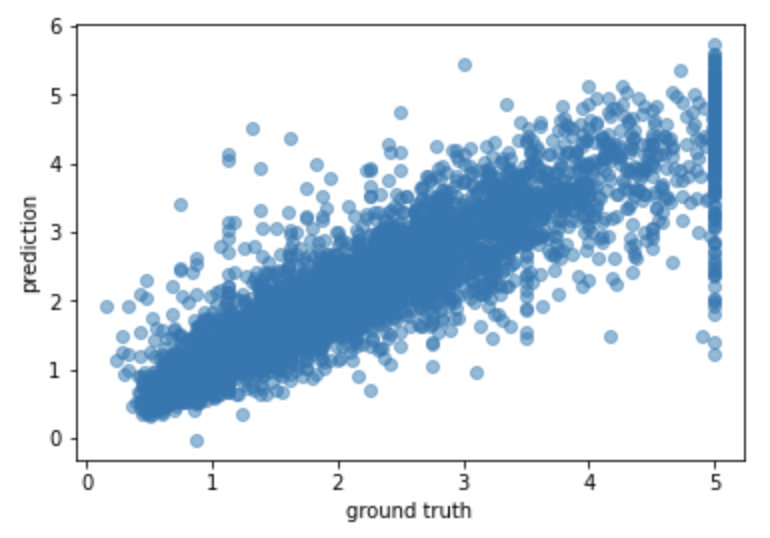
比較的綺麗に右上がりの線形が描けているように見えますが、Outlierが存在するかもしれませんね。業務であれば、Outlierを除外するかそのまま含めるかを判断しますが、今回はそのまま含めていきます。
3-3. Cross Validation / Performance tuning
では、Cross Validationをしつつ、Base modelを少しチューニングしてみます。今回はGridSearchCVで、5 Foldでcross validationを行います。また、max_depthとn_estimatorsをチューニングします。さらに、early_stopping_roundsを使用していきます。
In [14]: from sklearn.model_selection import GridSearchCV

In [15]: xgb_model4 = GridSearchCV(
    ...:                 estimator=XGBRegressor(),
    ...:                 param_grid={
    ...:                         'max_depth': [3, None],
    ...:                         'n_estimators': (10, 50, 100, 1000)
    ...:                 },
    ...:                 cv=5,
    ...:                 n_jobs=-1,
    ...:                 scoring='neg_mean_squared_error'
    ...:             )
    ...:
    ...: fit_params_reg = {
    ...:     'estimator__eval_metric': 'rmse',
    ...:     'estimator__early_stopping_rounds': 300,
    ...: }
    ...:
    ...: xgb_model4.set_params(**fit_params_reg)
    ...: xgb_model4.fit(X_train, y_train, eval_set=[(X_train, y_train)], verbose=0).best_estimator_

Out[14]:
XGBRegressor(base_score=0.5, booster='gbtree', callbacks=None,
             colsample_bylevel=1, colsample_bynode=1, colsample_bytree=1,
             early_stopping_rounds=300, enable_categorical=False,
             eval_metric='rmse', feature_types=None, gamma=0, gpu_id=-1,
             grow_policy='depthwise', importance_type=None,
             interaction_constraints='', learning_rate=0.300000012, max_bin=256,
             max_cat_threshold=64, max_cat_to_onehot=4, max_delta_step=0,
             max_depth=3, max_leaves=0, min_child_weight=1, missing=nan,
             monotone_constraints='()', n_estimators=1000, n_jobs=0,
             num_parallel_tree=1, predictor='auto', random_state=0, ...)
3-4. Prediction / Validation (ver2)
再度、validationデータを使用してPredictionを行い、Validationを行います。今回はValidation Scoreを前回と比較します。
In [16]: y_train_pred4 = xgb_model4.predict(X_train)
    ...: y_pred4 = xgb_model4.predict(X_test)
    ...:
    ...: print('Train r2 score: ', r2_score(y_train_pred4, y_train))
    ...: print('Test r2 score: ', r2_score(y_test, y_pred4))
    ...: train_mse4 = mean_squared_error(y_train_pred4, y_train)
    ...: test_mse4 = mean_squared_error(y_pred4, y_test)
    ...: train_rmse4 = np.sqrt(train_mse4)
    ...: test_rmse4 = np.sqrt(test_mse4)
    ...: print('Train RMSE: %.4f' % train_rmse4)
    ...: print('Test RMSE: %.4f' % test_rmse4)

Train r2 score:  0.9412675300402117
Test r2 score:  0.8395302864351717
Train RMSE: 0.2653
Test RMSE: 0.4625
Validation Scoreがやや上がったようでした。
今回はWeightですが、MedIncが一番多く使用されているようです。次は、Gainも確認してみようと思います。
In [17]: plt.scatter(y_test, y_pred4, alpha=0.5)
    ...: plt.xlabel('ground truth')
    ...: plt.ylabel('prediction')
    ...: plt.show()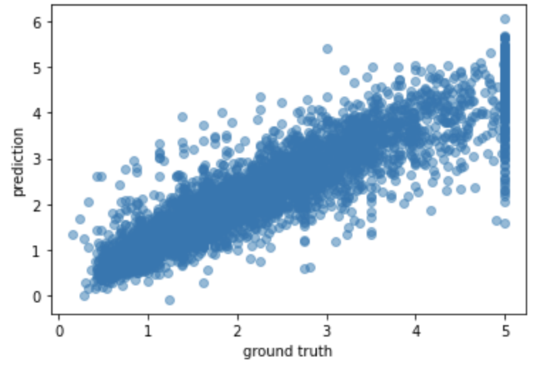
やや、ばらつきが収まっているようにも見えますが、Outlierの対応は必要のようです。
3.5 Feature Importance
念の為、Feature Importanceも確認してみます。model.best_estimator_をplot_importanceに渡しているのは、Gridsearchを使用したので、best estimatorをパラメータに設定しています。
In [18]: from xgboost import plot_importance
    ...:
    ...: plot_importance(xgb_model4.best_estimator_)
    ...: plt.show()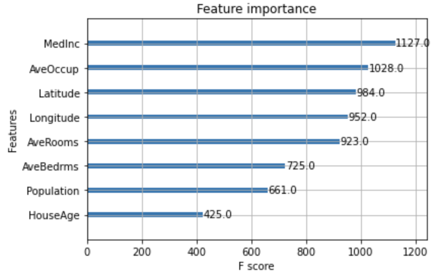
今回はWeightですが、MedIncが一番多く使用されているようです。次は、Gainも確認してみようと思います。
In [19]: plot_importance(xgb_model4.best_estimator_, importance_type = "gain")
    ...: plt.show()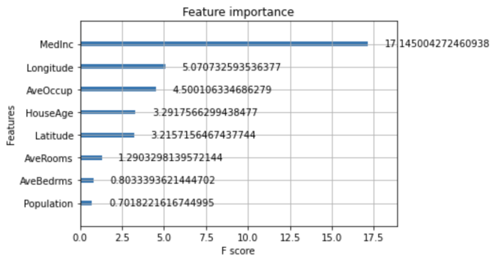
やはり、MedIncがKey featureなのかもしれません。
4. まとめ
ということで、今回は「Python – XGBoostで回帰分析(Scikit-learn)」について記載してみました。Causal Machine Learning特にEcomMLでは、scikit-learnのXGBoostを使用する必要もあったので、scikit-learnも使用する機会は結構あるのではないかと思います。