Python – XGBoostで回帰分析(XGBoost API)
今回は業務にて非常に使用する機会の多い、Python – XGBoostで回帰分析(XGBoost API)について記載していこうと思います。最近では、Causal Inferenceのmodelでもかなり頻繁に使用する機会が多いのではないでしょうか。そこで、今回は回帰/Regressionについて記載していきます。
Scikit-learn APIのXGBoostは以下をご参照ください。
1. データ準備
データ準備として、今回はsklearn.datasetsのcalifornia_housingを使用していきます。このデータは回帰用のSampleデータとして使用できますので、必要に応じて使用してみてください。また、pandas.dataframeを使用するので、pandasもimportし、sklearn.datasetsのcalifornia_housingのデータをpandas.dataframeに格納します。
In [1]: import pandas as pd
   ...: from sklearn.datasets import fetch_california_housing

In [2]: california_housing = fetch_california_housing()
   ...: df = pd.DataFrame(california_housing.data, columns=california_housing.feature_names)
   ...: df.head()

Out[2]:
   MedInc  HouseAge  AveRooms  AveBedrms  Population  AveOccup  Latitude  Longitude
0  8.3252      41.0  6.984127   1.023810       322.0  2.555556     37.88    -122.23
1  8.3014      21.0  6.238137   0.971880      2401.0  2.109842     37.86    -122.22
2  7.2574      52.0  8.288136   1.073446       496.0  2.802260     37.85    -122.24
3  5.6431      52.0  5.817352   1.073059       558.0  2.547945     37.85    -122.25
4  3.8462      52.0  6.281853   1.081081       565.0  2.181467     37.85    -122.25
california_housingのtargetデータ「MudHouseVal」をpandas.dataframeに追加してデータ準備完了です。
In [3]: df['MedHouseVal'] = pd.Series(california_housing.target)
   ...: df.head()

Out[3]:
   MedInc  HouseAge  AveRooms  AveBedrms  Population  AveOccup  Latitude  Longitude  MedHouseVal
0  8.3252      41.0  6.984127   1.023810       322.0  2.555556     37.88    -122.23        4.526
1  8.3014      21.0  6.238137   0.971880      2401.0  2.109842     37.86    -122.22        3.585
2  7.2574      52.0  8.288136   1.073446       496.0  2.802260     37.85    -122.24        3.521
3  5.6431      52.0  5.817352   1.073059       558.0  2.547945     37.85    -122.25        3.413
4  3.8462      52.0  6.281853   1.081081       565.0  2.181467     37.85    -122.25        3.422
以上でデータ準備は完了です。
2. Training / Validationデータ作成
では、TrainingデータとValidationデータを作成して、modelingの準備をしていこうと思います。
念の為、TargetデータにNaNが存在するかを確認してみます。
In [4]: df['MedHouseVal'].isnull().sum()

Out[4]:
0
特に前処理の必要はなさそうなので、そのまま変数yに代入していきます。
In [5]: y = df['MedHouseVal']次に、Feature setを変数Xに格納し、各カラムの要約統計量を確認してみます。
In [6]: X = df.drop('MedHouseVal', axis=1)
   ...: X.describe()

Out[6]:
             MedInc      HouseAge      AveRooms     AveBedrms    Population      AveOccup      Latitude     Longitude
count  20640.000000  20640.000000  20640.000000  20640.000000  20640.000000  20640.000000  20640.000000  20640.000000
mean       3.870671     28.639486      5.429000      1.096675   1425.476744      3.070655     35.631861   -119.569704
std        1.899822     12.585558      2.474173      0.473911   1132.462122     10.386050      2.135952      2.003532
min        0.499900      1.000000      0.846154      0.333333      3.000000      0.692308     32.540000   -124.350000
25%        2.563400     18.000000      4.440716      1.006079    787.000000      2.429741     33.930000   -121.800000
50%        3.534800     29.000000      5.229129      1.048780   1166.000000      2.818116     34.260000   -118.490000
75%        4.743250     37.000000      6.052381      1.099526   1725.000000      3.282261     37.710000   -118.010000
max       15.000100     52.000000    141.909091     34.066667  35682.000000   1243.333333     41.950000   -114.310000
また、Nullチェックも行います。
In [7]: X.isnull().sum()
Out[7]:
MedInc        0
HouseAge      0
AveRooms      0
AveBedrms     0
Population    0
AveOccup      0
Latitude      0
Longitude     0
dtype: int64
Nullもなさそうなので、Training / Validationデータを作成していきます。
In [8]: from sklearn.model_selection import train_test_split
   ...:
   ...: X_train, X_test, y_train, y_test = train_test_split(X, y, test_size=0.3, random_state=0)
今回は、7:3で作成していますが、業務に合わせて適宜変更することが必要だと思います。
3. XGBoostで回帰分析(XGBoost API)
それでは、本題の回帰分析を行なっていこうと思います。XGBoost APIのtrain()で回帰分析を行なってみます。scikit-learnでの回帰分析は別の記事にて行なってみようと思います。
3-1. DMatrix、Train実施
では、XGBoost APIでTrainingを行なってみます。まず、Core Data Structureにデータをセットしていきます。以下API docです。
https://xgboost.readthedocs.io/en/stable/python/python_api.html#module-xgboost.core
次に、XGBoostのLearning APIでtrainingを行います。また、精度向上のために、early stoppingを1000で実行していきます。なお、evaluation metricはRMSEを使用します。
https://xgboost.readthedocs.io/en/stable/python/python_api.html#module-xgboost.training
In [10]: from xgboost import DMatrix, train
    ...:
    ...: dtrain = DMatrix(X_train, label=y_train)
    ...: dtest = DMatrix(X_test, label=y_test)
    ...:
    ...: xgb_params = {
    ...:     'eval_metric': 'rmse',
    ...: }
    ...:
    ...: evals = [(dtrain, 'train'), (dtest, 'eval')]
    ...:
    ...: evals_result = {}
    ...: model = train(
    ...:             xgb_params,
    ...:             dtrain,
    ...:             num_boost_round=1000,
    ...:             evals=evals,
    ...:             evals_result=evals_result,
    ...:             verbose_eval = 100
    ...: )

[0]	train-rmse:1.44495	eval-rmse:1.45025
[100]	train-rmse:0.26120	eval-rmse:0.47802
[200]	train-rmse:0.19185	eval-rmse:0.47662
[300]	train-rmse:0.14826	eval-rmse:0.47655
[400]	train-rmse:0.11905	eval-rmse:0.47565
[500]	train-rmse:0.09425	eval-rmse:0.47566
[600]	train-rmse:0.07563	eval-rmse:0.47566
[700]	train-rmse:0.05981	eval-rmse:0.47586
[800]	train-rmse:0.04899	eval-rmse:0.47608
[900]	train-rmse:0.04038	eval-rmse:0.47636
[999]	train-rmse:0.03356	eval-rmse:0.47633
3-2. Early stoppingの学習状況
学習状況をplotしてみます。
In [11]: import matplotlib.pyplot as plt
    ...:
    ...: train_metric = evals_result['train']['rmse']
    ...: plt.plot(train_metric, label='train rmse')
    ...: eval_metric = evals_result['eval']['rmse']
    ...: plt.plot(eval_metric, label='eval rmse')
    ...: plt.grid()
    ...: plt.legend()
    ...: plt.xlabel('rounds')
    ...: plt.ylabel('rmse')
    ...: plt.show()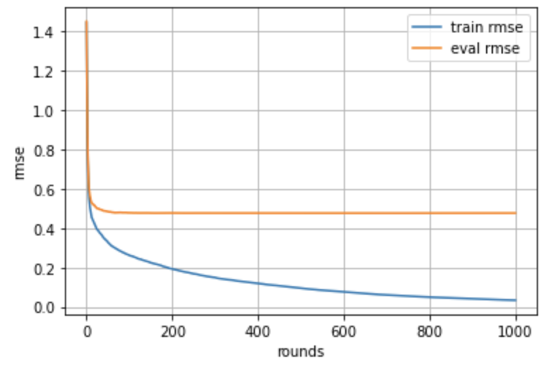
3-3. Prediction / Validation
では、Validationを行うために、validationデータを使用してPredictionを行い、Validation Scoreとして今回はRMSEを確認してみます。
In [12]: import numpy as np
    ...: from sklearn.metrics import mean_squared_error
    ...:
    ...: y_pred = model.predict(dtest)
    ...:
    ...: rmse = np.sqrt(mean_squared_error(y_test, y_pred))
    ...: print("RMSE : % f" %(rmse))

RMSE :  0.476332
Scatter plotを使用して分析結果を確認してみます。
In [13]: import matplotlib.pyplot as plt
    ...:
    ...: plt.scatter(y_test, y_pred, alpha=0.5)
    ...: plt.xlabel('ground truth')
    ...: plt.ylabel('prediction')
    ...: plt.show()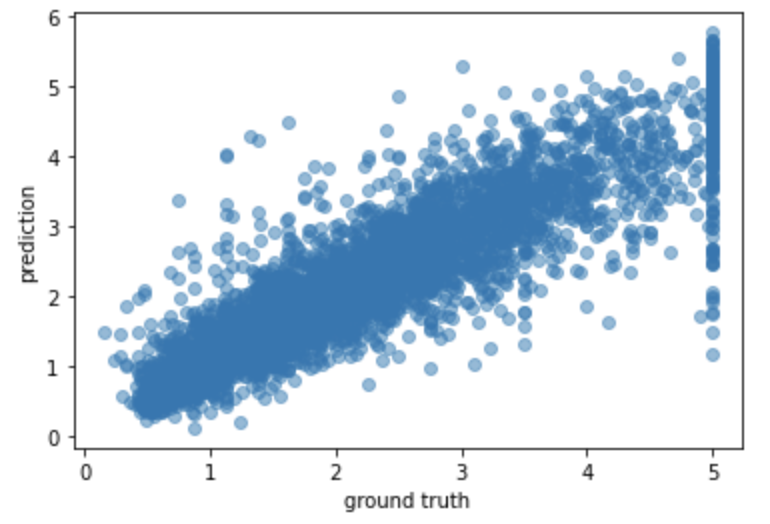
Outlierが存在するかもしれませんね。業務であれば、Outlierを除外するかそのまま含めるかを判断しますが、今回はそのまま含めていきます。
3-4. Feature Importance
では、Feature Importanceも確認していきます。
In [15]: from xgboost import plot_importance
    ...:
    ...: plot_importance(model)
    ...: plt.show()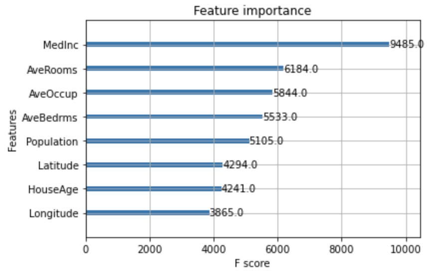
今回はWeightですが、MedIncが一番多く使用されているようです。次は、Gainも確認してみようと思います。
In [16]: plot_importance(model, importance_type = "gain")
    ...: plt.show()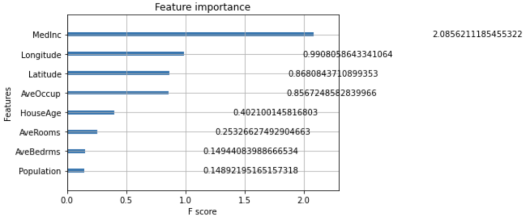
やはり、MedIncがKey featureなのかもしれません。
4. まとめ
ということで、今回は「Python – XGBoostで回帰分析(XGBoost API)」について記載してみました。ただ、Causal Machine Learning特にEcomMLでは、scikit-learnのXGBoostを使用する必要もあったので、次回はscikit-learnで回帰分析を行なってみようと思います。